Makaleyi Türkçe okumak için

SAGe!

In this post, you will read the summary and explanations I prepared foor my presentation dated August 6, 2026, where I presented the article SAGe: A Lightweight Algorithm-Architecture Co-Design for Mitigating the Data Preparation Bottleneck in Large-Scale Genome Sequence Analysis.

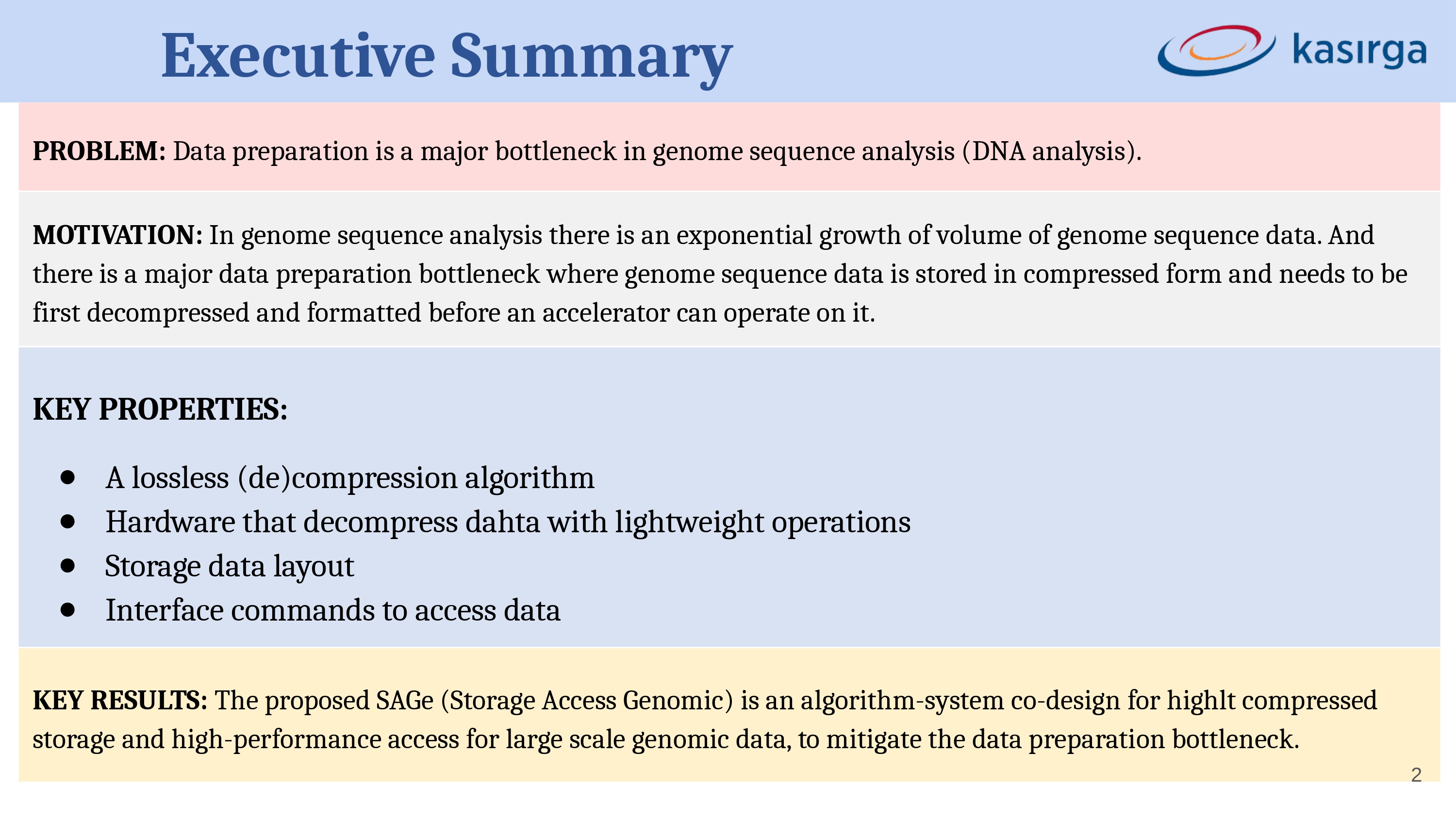
Welcome to this article about the SAGe paper and system, which is a solution developed for the data preparation stage that causes a bottleneck in genome sequencing, meaning DNA analysis.

The problem, as you can see in the visual above, is that there is a serious bottleneck in the data preparation stage in gene analysis.

Their main motivation is: New data is being added to closed or open-source gene pools every day, and these need to be processed when necessary. Since genome data takes up a lot of space in memory, it needs to be stored in a compressed format, and when required, it must be easily decompressed from its compressed state to its normal state and processed.

To develop a suitable solution for this problem, there are some basic requirements; these are:

• Lossless compression (zip) and decompression (unzip),
• Restoring the data from its compressed state to its original state with simple operations,
• The existence of a storage template,
• Specific interface commands to access the data.

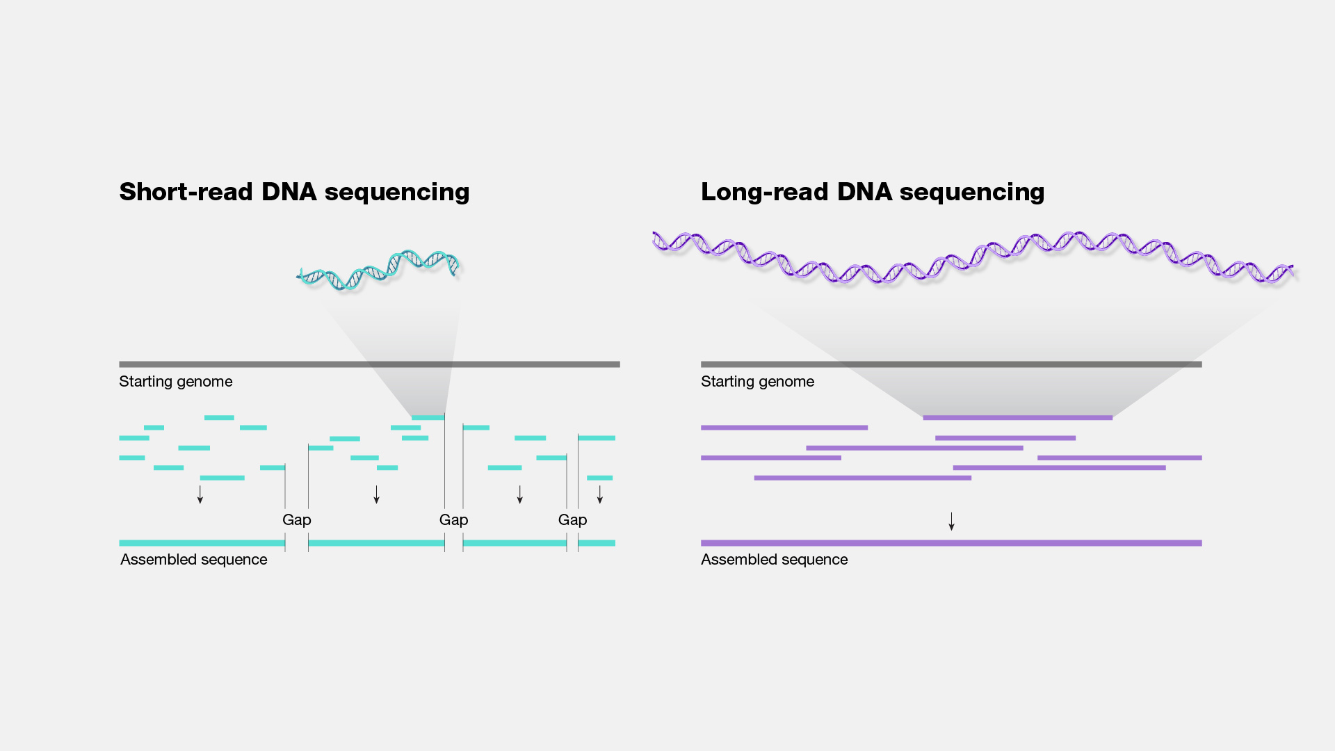
Today's genome analysis tools cannot analyze a DNA from beginning to end. Therefore, the analysis process takes place in small pieces called "reads". These "reads" are not sequential pieces but pieces of a certain length read from random points. So, some "reads" might contain the same genes. Because they can overlap.

First, we can look at this graph of the bottleneck in the data preparation stage, which is the main problem the article tries to solve.

Introduction

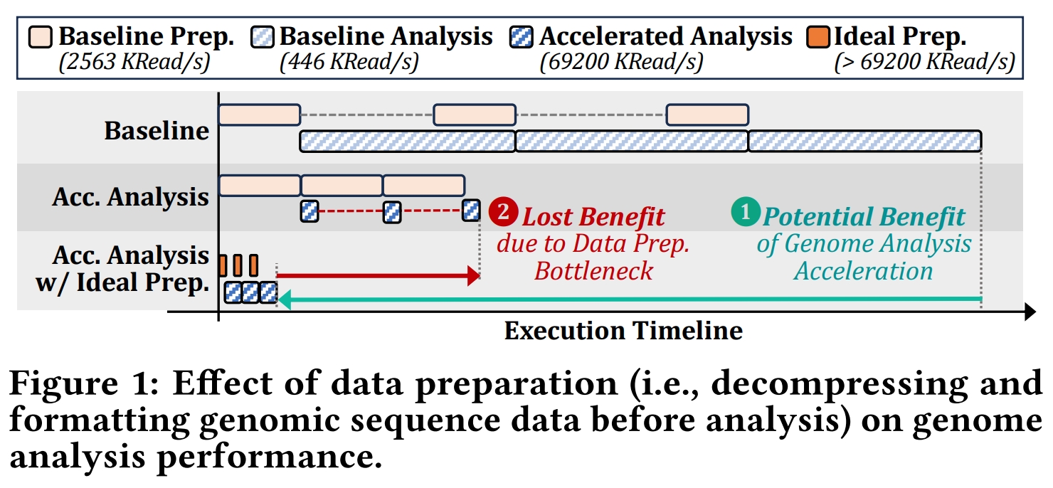
Baseline represents current data analysis and data compression software,

Acc. Analysis represents hardware-level data analysis and the same data compression software as Baseline,

the Ideal part represents both hardware-level data analysis and the most ideal data compression level possible.

Background

If we examine the data flow:

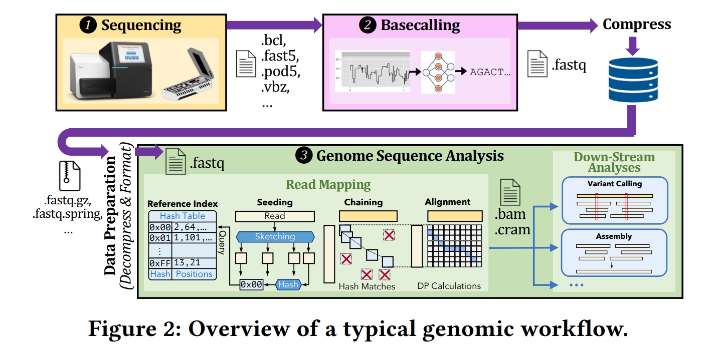
In the Sequencing part, devices called sequencers read the DNA and convert it into digital signals. But as I said just before, this reading process cannot be done from beginning to end. Instead, it is read in "reads".

In the Basecalling part, digital signals are converted into strings in "FASTQ" format, which makes up 75.9 percent of open-source data as of October 2025 ¹. Here, in addition to the ATGC alphabet (Adenine, Thymine, Guanine, Cytosine), "N" is also used for signals that cannot be detected with enough accuracy rate.

Also, a quality score is kept for each nucleotide, which is a value that expresses how confident the algorithm is that the incoming signal represents that nucleotide.

Then, all data is compressed to save space and transmitted to the genome analysis process.

In the Genome Analysis part, before the data is processed, it is converted from its compressed state to its normal state (unzip) and is first put through the stage we call Read Mapping, where it is determined which part of the gene the incoming "reads" correspond to.

Finally, the located data can be formatted for various analyses and put into processing.

Generally, the Genome Analysis part is done with "read sets" that have previously gone through the Sequencing and Basecalling stages because a "read set" needs to be analyzed repeatedly several times in a row or at different times to increase accuracy.

The bottleneck that the article is trying to solve is actually exactly in this genome analysis part.

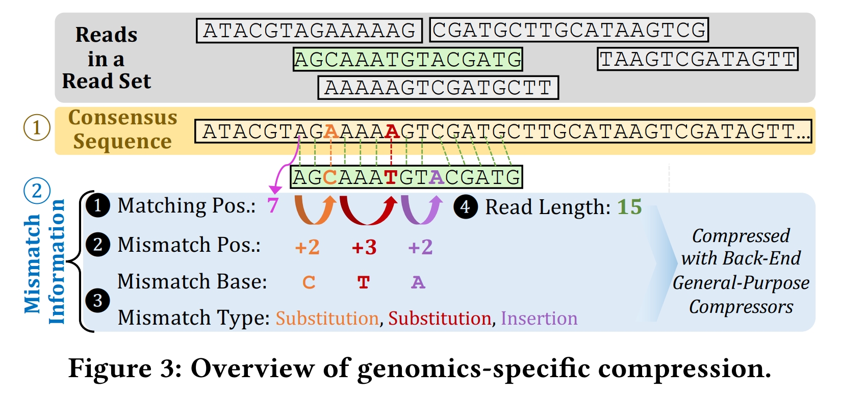
There are several methods for compressing data. But generally, in the field we are talking about right now, genome-specific compression techniques are used. The difference between these and classical compression techniques is that they can detect long similarities in DNA data and perform more effective compression.

In the Genome-Specific Compression used by the article, incoming "read sets" are compared with a consensus sequence (we can call this the sequence that is accepted as correct).

And 4 main features are recorded:

• Matching position: From which sequence of the Consensus Sequence the "read set" matches.
• Mismatch positions: Data on how many sequences after the matching position or the previous mismatch position the mismatch occurred, and what type of base is incorrect.
• The type of error: Such as mismatched base, extra detected base.
• And the total length of the "read set".

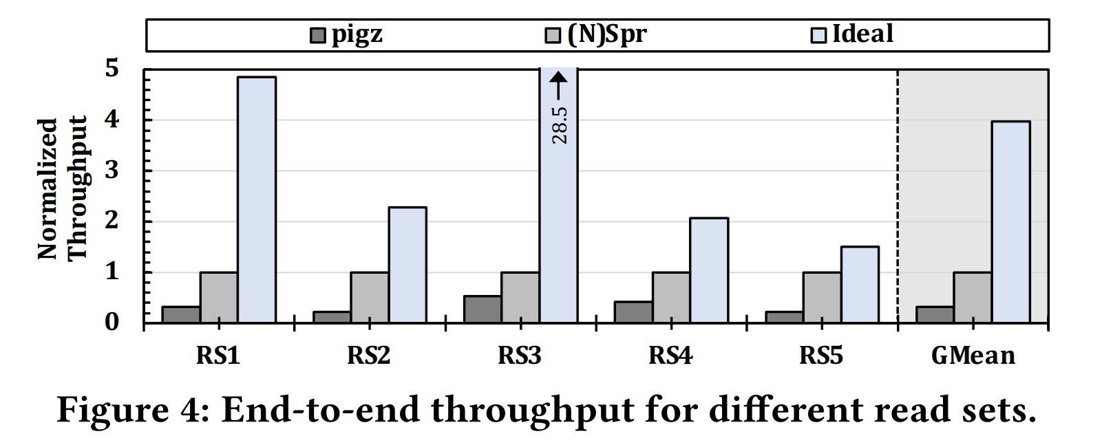
In this graph, three different methods selected for the data preparation part are shown. For the analysis part after data preparation, they commonly used a modern hardware accelerator for all of them. So, the comparison in this graph is only for the data preparation part.

pigz: A general-purpose compression technique; it is not something specialized for genome data.

N(Spr): A modern, software-based compression technique specialized for genome data.

Ideal: A situation assumed to be perfect that does not exist in reality. It expresses the situation where the process of decompressing the compressed data happens instantly, meaning it takes 0 seconds. Actually, this ideal situation evaluates the state where the bottleneck completely disappears.

As can be seen here, the preparation of data significantly affects the overall performance.

By the way, all the methods mentioned in this data preparation part are based on decompressing compressed data because the size of the data being worked on is very large, and storing it without compression is inefficient. Even storing only the data to be used without compression is inefficient because, as I mentioned just before, a "read set" is generally processed more than once.

After this part, they moved forward together with the other works of the team that wrote this article (GenStore ²), and they mostly talked about NDP, that is, Near Data Processing. This actually means that all these data preparation operations are done on memory inside an SSD.

What is SAGe?

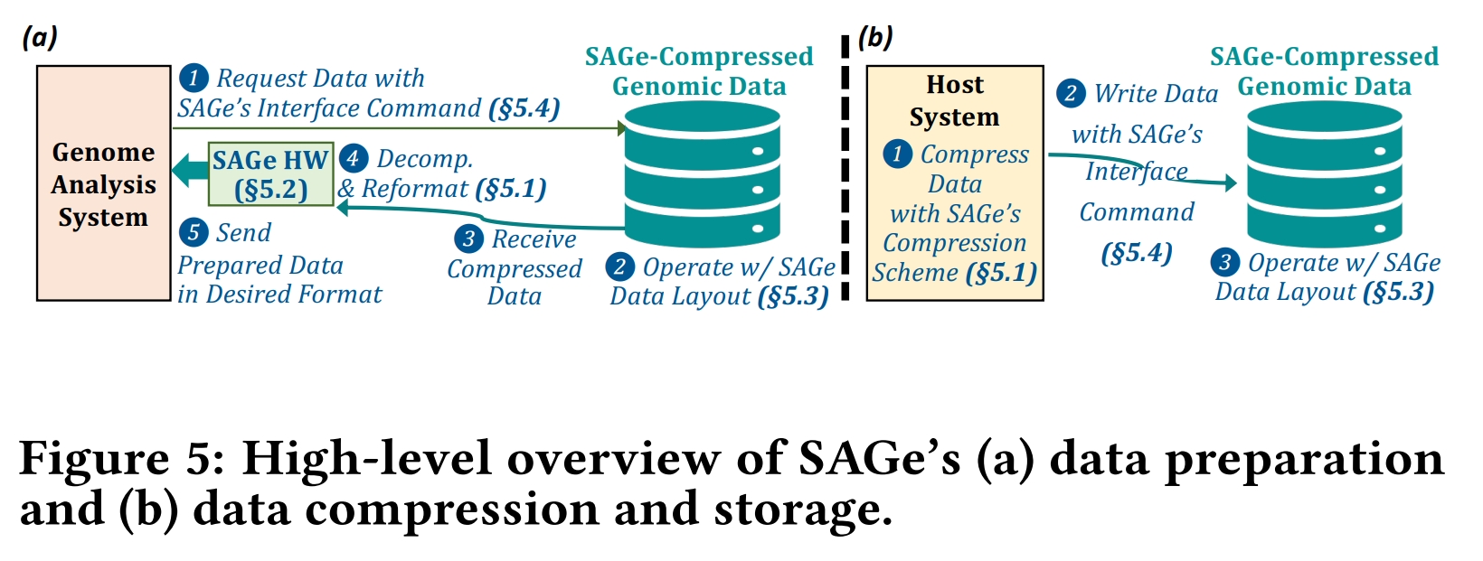
Moving on to the SAGe algorithm and hardware-integrated system proposed by the article. Here, they prioritized the 4 basic features I mentioned at the very beginning of the presentation.

SAGe's general data preparation logic is as follows, as seen in part a:

• The genome analysis system requests the data with SAGe's interface commands.
• Then, SAGe starts performing its operations in accordance with its own data schema.
• First, it takes the compressed data from memory and, thanks to its own mechanisms, decompresses the data and restores it to its normal state.
• And it transmits the data to the genome analysis system.

In the data compression phase, that is, in part b:

Since the compression of the data is not on the critical path and does not cause a bottleneck, the compression process occurs directly in the upper units but using SAGe's compression schemas. And it is stored in the relevant place with SAGe's interface commands.

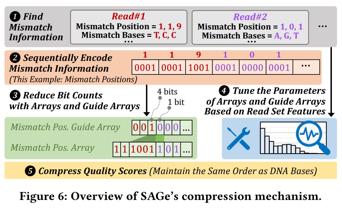
After the external working logic, let's look at the truly important part, which is how SAGe compresses the data.

The most fundamental feature that distinguishes SAGe from other genome data-specific compression techniques. Identifying mismatches during compression and compressing them in a suitable arrangement.

As I mentioned before and as seen in this diagram, SAGe basically keeps 3 features:

• Mismatch position,
• The type of the mismatched base,
• The location where the first base of the "read set" first matches the real data.

Then SAGe records the mismatch position data sequentially in a bulk array. And it keeps track of which of these data are of what length with a guide array.

The main reason why SAGe can use a guide array is that mismatches in "read sets" generally occur at fixed intervals, and the number of various intervals is limited. So, for instance, if we look at this example, mismatches occurred every 1 or 9 bases. Therefore, a record could be made in the guide array as 0 for 1, and 1 for 9.

In this way, both space is saved and lossless compression is achieved.

"Quality scores" are also compressed with a similar method, but this was kept optional because some of the machines performing the sequencing process raise accuracy to a very high level, so they do not produce "quality scores". Most genome analysis environments no longer use "quality scores" anyway.

Huffman Coding Example ³

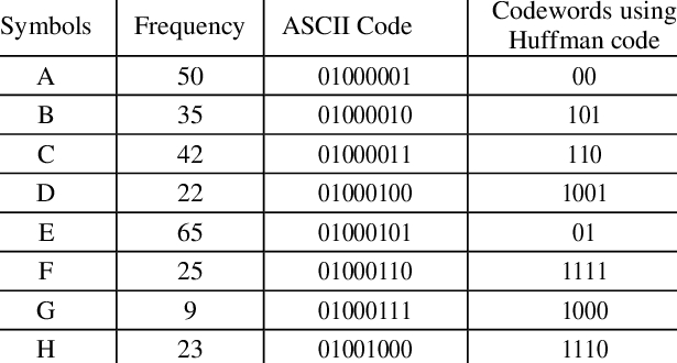
SAGe minimized the length of the mismatch position and guide array using an algorithm similar to the Huffman Algorithm ^{4 5}. In this process, space is saved by expressing the number we encounter the most, meaning the one with the highest frequency, with the fewest bits.

The algorithm which presented in the article:

Input: Histogram of mismatch position bit counts H, where |H| ≤ 32, and a tuning convergence threshold ε.

Output: List of bit counts W for encoding mismatch positions.

ℓmin ← ∞ ▷ Initialize min. encoding size
x0 ← 0
for all d ∈ {1, . . . , 8} do ▷ Find optimal |W|.
	ℓlast ← ℓmin ▷ Best result from previous d values
	for all (x1, . . . , xd) ∈ |H|^d s.t. x0 < x1 < · · · < xd do
		ℓ ← total length of encoded mismatch positions and guide arrays s.t. positions with bit counts ∈ (xi, xi+1] are encoded with xi+1 bits.
		if ℓ < ℓmin then
			ℓmin = ℓ
			W ← (x1, . . . , xd)
	if (ℓlast − ℓmin)/ℓmin < ε then
		break ▷ Exit loop when ℓmin converges, typically at d < 8
return W

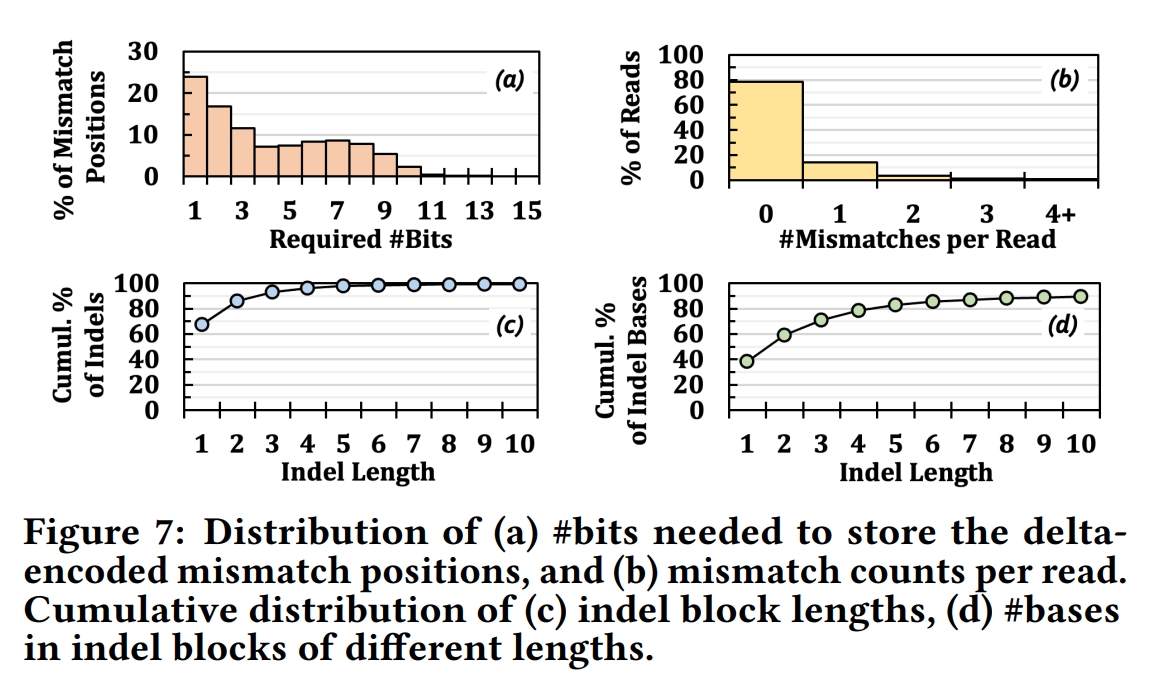
As can be seen in graph A, it is obvious that we can save space if we use a small number of bits for error positions with high frequencies.

As can be understood from graph B, mismatch is actually not a very frequently encountered situation because tests were generally conducted on short "reads", and the error rate in short "reads" is much less compared to long "reads". However, since "reads" can contain the same genes overlapping, short "reads" cause a loss of space.

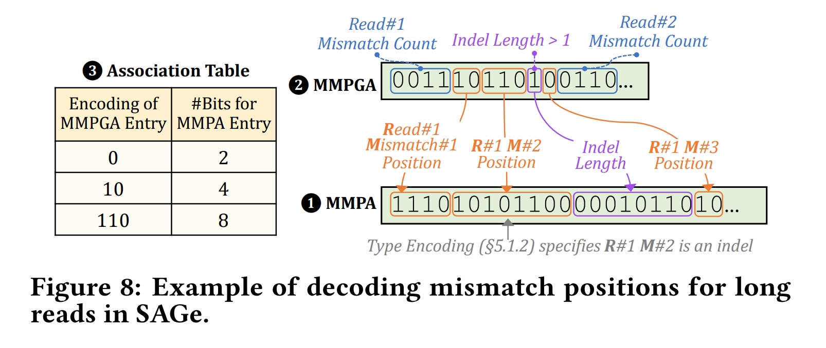
In the process of decompressing the compressed data,

SAGe first looks at the guide array and learns how many mismatches there are in that "read". Then, it continues reading in the same array and sequentially learns the length of the binary number where the position of each mismatch is kept, and reads that length of numbers in the mismatch position array.

Sometimes insertion or deletion errors occur within a "read". SAGe divided these into two as those with a length greater than 1 or those with a length of 1, and always kept the length of those greater than 1 in 8 bits.

Edge Cases

They also optimized SAGe for several edge cases.

The first of these is that in some situations where it is not clearly understood which base it is for the alphabet consisting of 4 basic bases as ATGC, a letter named "N" needs to be added; this requires expanding the alphabet to 3 bits when it could be kept in 2 bits.

To solve the identification of edge cases, they marked the arrays containing "reads" with unidentified bases by making their first character 0. In this way, it was determined that that array is an array containing an edge case, and they didn't have to use a 3-bit alphabet for all "reads".

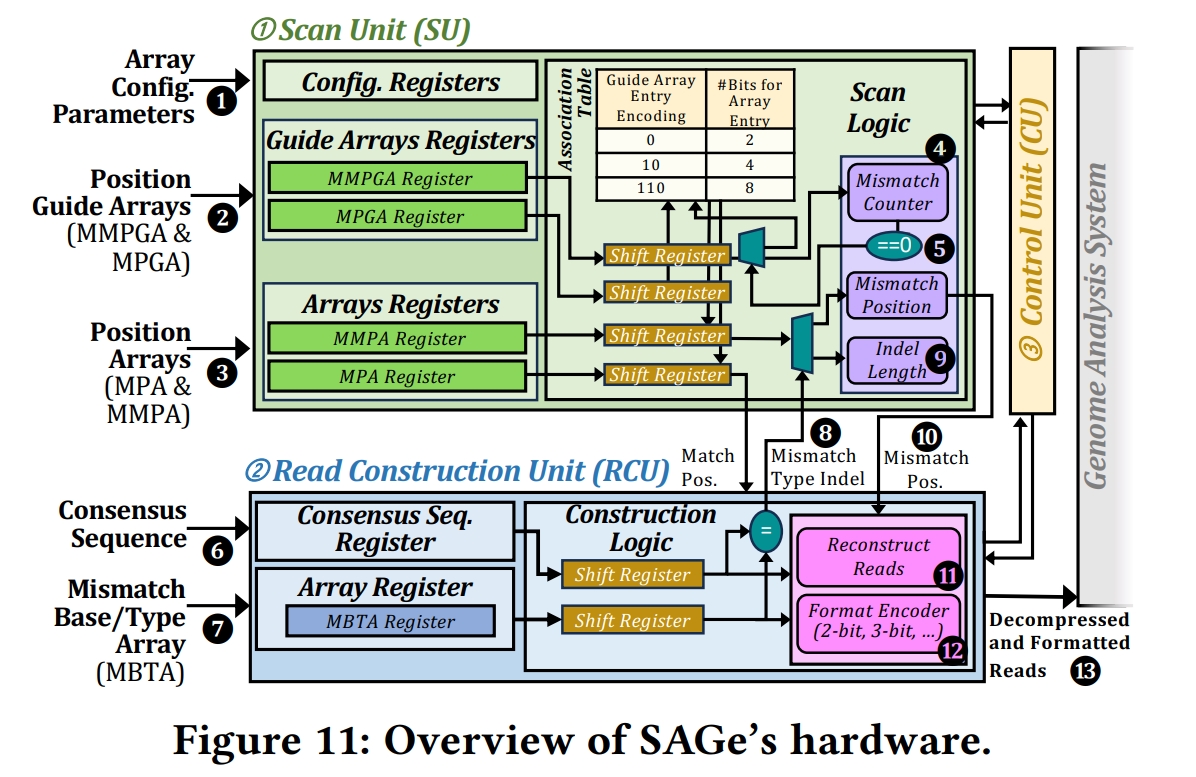
Moving on to SAGe's hardware system

SAGe's hardware system consists of 3 main parts.

Scanning Unit: It determines mismatches using the mismatch array and the guide array.

Then it transmits the data to the "Read" Generator Unit, and in this part, "reads" are reconstructed by taking them out of the compressed format.

The Control Unit controls all these operations.

In light of the operations in this diagram, the decompression operations I just described take place via hardware.

One of the strongest features of the SAGe hardware is that this Scanning Unit and "Read" Generator Unit I mentioned process the incoming data immediately with streaming access without needing large buffers and move on to the next operation without needing extra memory space. Because SAGe keeps mismatch positions in order of arrival, it can easily perform sequential operations.

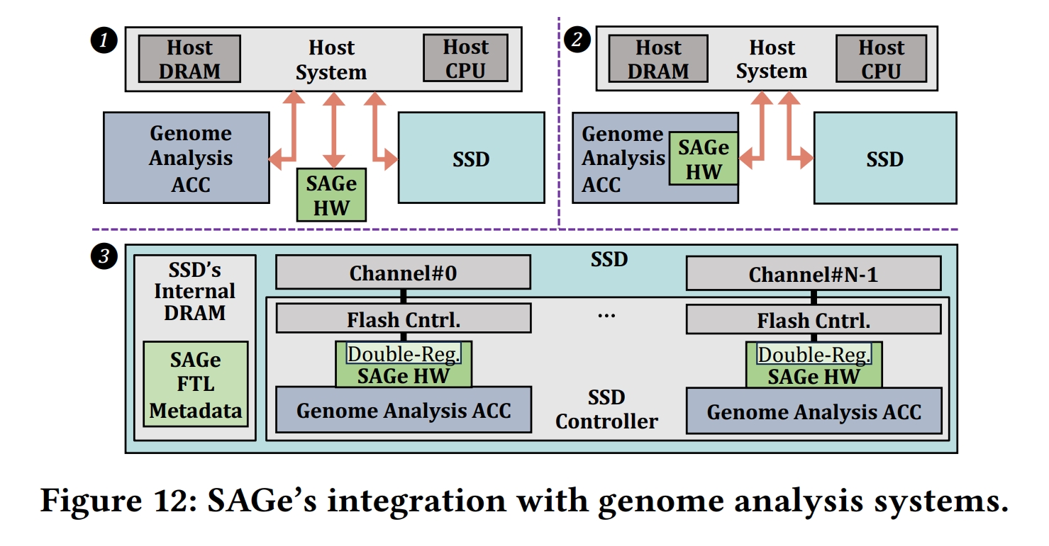
SAGe can be integrated into systems in 3 different ways.

The first way is connecting SAGe directly to the main system with various protocols.

The second way is placing it inside the accelerator like a peripheral, with the accelerator's input and output being done with SAGe.

The third way is placing it directly inside an SSD using NDP, that is, Near Data Processing.

In cases where SAGe is used inside an SSD, it marks all data as genomic and non-genomic so that the SSD can be used for other purposes as well; this way, the SSD can be used for other purposes while it is integrated with SAGe.

Evaluation

Methods Used in the Evaluation of SAGe

They implemented the logical elements of SAGe with Verilog, created a DRAM with Ramulator 1.0, then set up the internal operations of the SSD with MQSim, and performed a performance test on a 1.5-terabyte DRAM with 128 cores and 256 hardware threads.

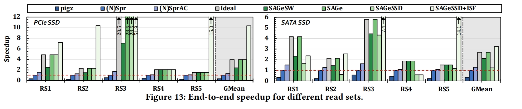
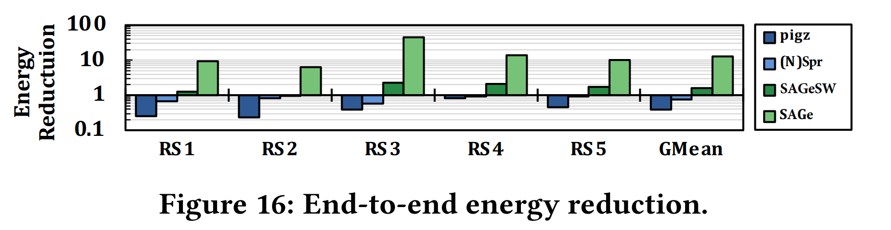
SAGe showed a significant speed increase and caught up with the Ideal operation, which can do the decompression (unzip) operation we call ideal in 0 seconds, meaning instantly, in terms of speed. The main reason it achieved this is that it removed the decompression (unzip) operation, which is the real bottleneck in the genome analysis application, from being a bottleneck. In this way, since this operation is not on the critical path, it provides a serious increase in speed. However, this situation of being saved from the bottleneck is only valid for hardware implementations of SAGe; even though there is an acceleration in its software implementation, it could not be saved from the bottleneck.

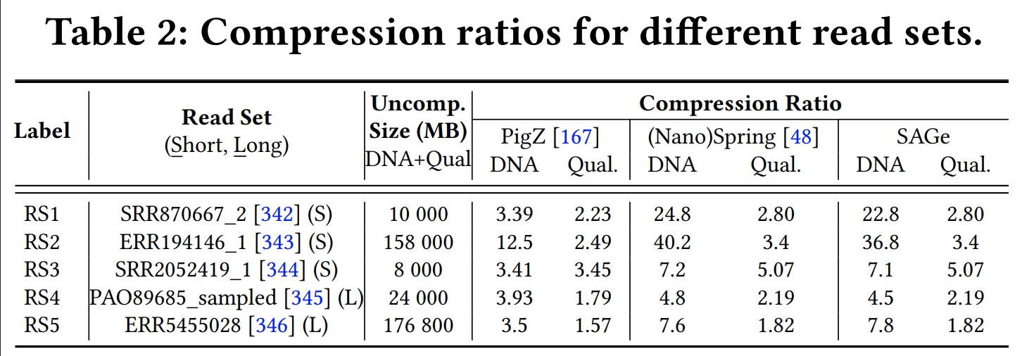
In terms of compression size, it performed a compression that is about 3 times better than pigz, which is not specialized for genome data, and quite close to (N)Spr, which is specialized for genome data.

A Journeyman's Review

Simply, they did a par excellence work.

Not only did it break the main bottleneck in genome data compression and take the (unzip) operation off the critical path, but it also provided improvements at a certain level in terms of speed, compression ratio, and space utilization.

The algorithm could be improved by adding a few more parameters (I didn't dwell on this much in my article.).

There are also minor oddities in the writing of the article, but these are not something I focused on either.

Acknowledgements

Thank you for reading. I hope this writing made it easier for you to understand this paper and a few basic concepts and situations in genome analysis in general.

Have a good day. May your work feel fluent.

References

- Eric W Sayers, Jeffrey Beck, Evan E Bolton, J Rodney Brister, Jessica Chan, Ryan Connor, Michael Feldgarden, Anna M Fine, Kathryn Funk, Jinna Hoffman, Sivakumar Kannan, Christopher Kelly, William Klimke, Sunghwan Kim, Stacy Lathrop, Aron Marchler-Bauer, Terence D Murphy, Chris O’Sullivan, Erin Schmieder, Yuriy Skripchenko, Adam Stine, Francoise Thibaud-Nissen, Jiyao Wang, Jian Ye, Erin Zellers, Valerie A Schneider, and Kim D Pruitt. Database resources of the National Center for Biotechnology Information in 2025. Nucleic Acids Research, 2025. ↩
- Nika Mansouri Ghiasi, Jisung Park, Harun Mustafa, Jeremie Kim, Ataberk Olgun, Arvid Gollwitzer, Damla Senol Cali, Can Firtina, Haiyu Mao, Nour Almadhoun Alserr, Rachata Ausavarungnirun, Nandita Vijaykumar, Mohammed Alser, and Onur Mutlu. GenStore: A High-Performance in-Storage Processing System for Genome Sequence Analysis. In ASPLOS, 2022. ↩
- Huffman Coding Example ↩
- Geeksforgeeks Huffman Coding ↩
- Huffman Coding Wikipedia ↩